![<?echo $_SERVER['SERVER_NAME'];?>](/template/twentyseventeen/skin/images/header.jpg)
introduction
Reverse engineering computer-aided design (CAD) modeling refers to digital measurement of physical prototypes by means of laser scanners, etc., to obtain discrete point cloud data reflecting the surface of the object, that is, the three-dimensional coordinates of the physical surface, and then adopt parameters based on features and constraints. The modeling method is used to complete the CAD model reconstruction process. The reconstructed CAD model should reflect the shape characteristics of the physical surface.
Usually, product design generally follows the principle from 2D to 3D, and the sketch outline of most parts is a plane composite curve composed of straight lines, arcs and splines, and then processed by stretching, rotating and scanning. Surface. Therefore, reverse engineering CAD modeling for discrete point clouds is implemented using the following methods:
1) using a set of planes to process discrete point cloud slices to obtain a series of cross-sectional contour points;
2) Using constrained optimization fitting to obtain a section sketch curve set;
3) Reconstruct free-form surface features such as stretching, rotation, and scanning from these cross-section sketch curves.
Combined with the parametric design of the 2D sketch in the forward modeling system, the sketch curves do not exist in isolation, and they contain various geometric constraints, such as parallel lines and tangent lines. Similarly, in reverse engineering, the processing of the section sketch not only satisfies the approximation error with the data points, but also satisfies the constraint requirements of mutual questions.
Werghi et al. conducted in-depth research on the fitting of point cloud data by multiple plane and quadratic synchronization constraints, and established an overall framework for incorporating geometric constraints into reverse engineering. The constrained optimization problem is transformed into an unconstrained optimization problem, and the LM method is used to optimize the iterative solution. BenkÇ’ et al. also made a related research on the constraint fitting problem in reverse engineering. Each constraint was expressed independently, and the Lagrangian multiplier method was used to solve the optimization problem. Considering the redundant constraints and contradictory constraints that may be included in reverse engineering modeling, a numerical algorithm that can resolve the conflict between constraints is further given. Gong Youping proposed a new method of constraint solving. For the first time, the homotopy method was used to solve the surface fitting problem under constraint conditions in reverse engineering, and the size of the equation to be solved was reduced by constrained merging and the calculation speed was accelerated.
Currently, many forward-designed CAD software provides tools and API interfaces for secondary development. The software is re-developed by VB, C/C++ and other programming languages, so that the fusion reverse design module is added on the basis of the existing modeling functions of the CAD software, so that the reverse engineering CAD model reconstruction is realized. As a powerful 3D modeling software, SolidWorks software has rich 2D sketch curve design, analysis and editing functions, especially the curvature calculation of the curve and the modification and adjustment of the spline curve. At the same time, the software itself can quickly add various constraints between the curves and perform constraint management to avoid over-constraints, under-constraints and contradictions. Therefore, using SolidWorks software as the development and implementation platform of the constraint optimization technology for cross-section sketch curve in reverse engineering, the constraint management function and sketch design function of the software can be used to realize the cross-section sketch curve reconstruction based on point cloud slice data. Applying this method is beneficial to improve the reconstruction efficiency of the model and enhance the ability of reverse engineering to support product modification and innovation.
1 Fitting model of cross-section sketch curve and constraint expression
In the mechanical parts of the regular structure, most of the section sketch curves are curved loops (sections) composed of straight and circular segments connected end to end, and free curve segments are also included in irregular structural parts such as steam turbine blades. . Therefore, this paper will use the straight line, arc and free curve as the main research object of cross-section data processing, while the free curve is expressed by cubic B-spline curve.
1.1 Fitting expression of profile profile data
The most commonly used curve fitting method in the engineering field is the least squares method. By minimizing the sum of the squares of the errors, a linear system of equations is obtained, and a linear fitting equation can be solved to construct a fitting curve. Using the least squares method to fit a set of data points, the best results can be obtained. However, the complexity of the mathematical model will be different depending on the expression of the curve objective function. When using the least squares fitting with Euclidean distance, the mathematical model The constraint expression equations between the curves and the curves are very complicated. Especially when the discrete data volume is large and the shape is complex, the data segmentation fitting and smoothing are needed, which brings many difficulties to the calculation process. Therefore, BenkÇ’ uses the minimum of the algebraic distance sum as the objective function to simplify the fitting equation and improve the efficiency of the solution. In this paper, when the least squares fitting is performed on the cross-section contour points, the algebraic equation is used to express the curve features, and the minimum of the algebraic distance sum is taken as the fitting target, so that the unified equation is constructed to express the curve equation of the cross-section data as the fitting problem. The algebraic equations for each curve feature are expressed as follows.
Straight line: L(x, y) = l0x + l1y + l2 = 0, l0, l1, l2 are parameters of the linear equation, and the constraint condition l02 + l12 = 1 is satisfied.
Arc: C(x, y)=C0(x2+y2)+c1x+c2y+c3=0, c0, c1, c2, c3 are parameters of the arc equation and satisfy the constraint c12+c22-4c0c3- 1=0.
The B-spline curve S(u) is:
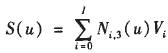
Where: Vi is the i-th control vertex; Ni, 3(u) is the basis function of the cubic B-spline curve; I+1 is the total number of control points; u is the node vector, u={u0, u1,..., uM }, M is the total number of nodes.
Under the above expression, the distance from the cross-section data point to the curve is the value obtained by substituting the coordinates of the point into the equation. Taking the least squares fitting of straight lines and arcs as an example, the objective function of least square fitting for J+1 data points is as follows.
The line is:
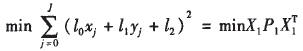
Where: X1 is a linear parameter matrix (l0, l1, l2); P1 is a linear separation matrix composed of data points, that is, P1=, D1=(xi, yi, 1); J+1 is the total number of data points.
The arc is:

Also converted into a matrix form: minX2P2XT2
In the formula, X2 is the parameter matrix of the toilet arc (Co, c1, c2, c3); P2 is the arc separation matrix composed of data points, that is, P2==[(xj+yj)2, xj, yj, 1].
Cubic B-spline curves are widely used in current CAD software. J+1 data points q0, q1, ..., qJ (J>I) are known. Curves are usually used to construct spline curves. The approximation curve generated by the method generally does not pass through the data points. Here you need to find a cubic B-spline curve:
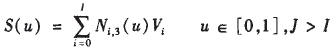
The curve satisfies q0=S(0), qJ=S(1); the remaining data points are approximated in the least squares sense, ie the objective function, f= is about the control vertex Vi(i=0,1,2,... , a minimum of I).
Figure 1 shows a simple example of a cubic B-spline curve for least squares fitting of data points. Given 17 data points (J = 16), the least squares approximation of the data points is performed with 11 control vertices.
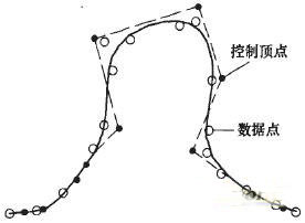
Figure 1 Three-B-spline curve for least squares fitting of data points
1.2 Constraint expression between section sketch curves
In reverse engineering, geometric constraints can be divided into internal constraints and external constraints. Internal constraints reflect specific geometric characteristics, such as the normalized constraints of lines and arcs; external constraints express the position of geometric shapes and geometric topological relationships, such as the distance between two parallel lines. General constraints (such as vertical constraints, tangency constraints, etc.) consist of constraint types, constraint objects, constraint points, and constraint expressions. For example, two linear vertical constraints, the constraint type is a vertical type, the constraint object is the two lines acting on the constraint, the constraint point is a vertical point, and the constraint is expressed as a constraint equation corresponding to the constraint type, as shown in Table 1. Figure 2 lists the types of geometric constraints between several common section sketch curves. The constraint types between each feature curve unit are mainly to satisfy the tangency constraint.
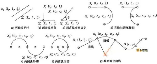
Figure 2 Geometric constraint types between common section curves
Table 1 lists the common geometric constraint types and their corresponding constraint equations for each of the fitted feature elements of the section sketch curve, mainly to satisfy the tangency constraint. The two straight line segments are represented as X1 (l0, l1, l2) and X'1, (l'0, l'1, l'2), and the two arc segments are respectively represented as X2 (c0, cl, c2, c3). And X'2 (c'0, c'1, c'2, c'3), the B-spline curve is represented by S(x, y). A line tangent to a B-spline curve can be expressed as two constraints:
1) The straight line L intersects the B-spline curve at the tangent point,
2) The straight line L and the B-spline curve are continuous at the tangent of the tangent point. At this point, you need to add an auxiliary point T1 (xT1, yT1), which is the tangent point of the two curves.
The tangent constraint between the arc C and the B-spline curve is expressed as:
1) The arc C and the B-spline curve intersect at the tangent point,
2) The circular arc and the B-spline curve are continuous at the tangent of the tangent point. The tangent point is recorded as T2 (xT2, yT2). Usually constraints have one or two constraint objects, and some constraints have no constraint points, such as parallel constraints.
Steel Bolt,Threaded Rod,Stainless Steel Bolts,Stainless Steel Anchor Bolts
Taizhou Risco Stainless Steel Products Co.,Ltd , https://www.riscofastener.com